.md .pdf

repository open issue

Contents

2. Inputs

2.1. Data Section

2.1.1. Heat Producers and Heat Storage – Tab

In this tab, the created or uploaded heat generator and heat storage data is shown in two tables (heat storage table and heat generator table). Fig. 2.26 shows the initial page (no heat generators and no heat storages are defined).

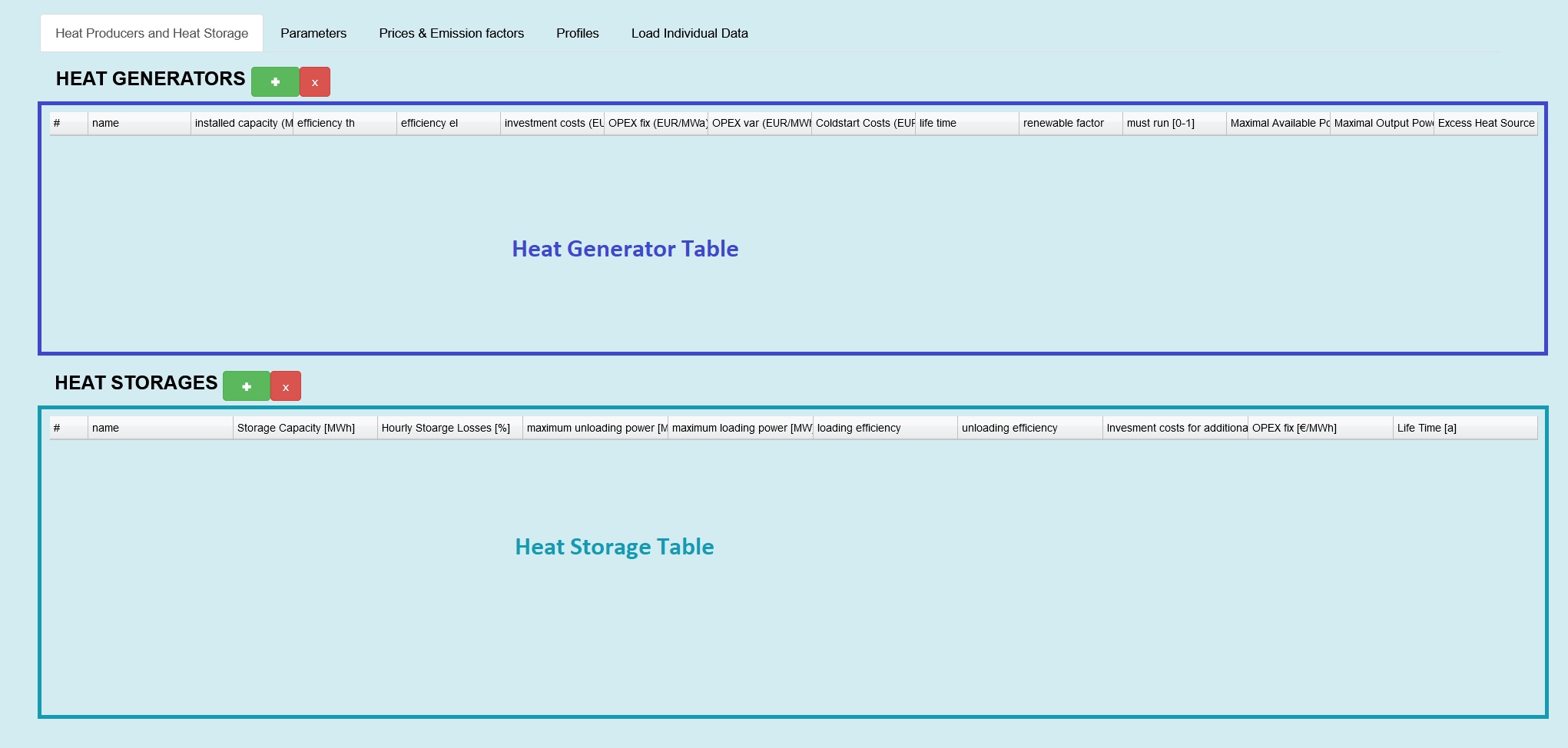
Fig. 2.26 Heat Generator and Storage Table

Note

Please notice that it is possible to edit the values in the tables.

By pressing the + button you will be able to add new heat generators or heat storages. This kind of adding tab pops up between the button section and the output section, see Fig. 2.27 and Fig. 2.28.

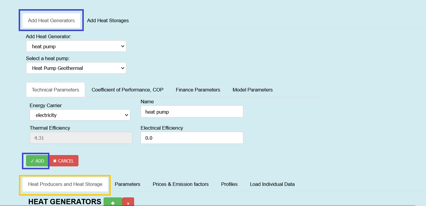
Fig. 2.27 Adding heat generators

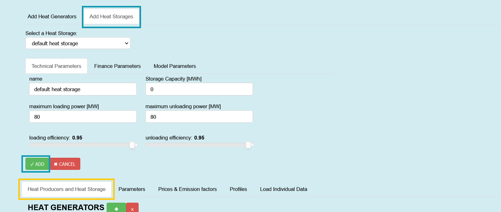
Fig. 2.28 Adding heat storages

• Heat Generator Table

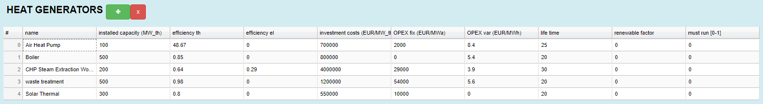
Fig. 2.29 Added heat generators in heat generator table

Your added, by pressing the + button) or uploaded data of heat generators is shown here, like in Fig. 2.29. You have the opportunity to change the values of the table below, but pay attention to the warning below!

These parameters can also be changed via uploading. Therefore, you have to create an excel sheet with the structure as described in The Web User Interface (subchapter Button Section). Then the parameters must be specified in the Heat Generators worksheet.

column name	format	unit	description
name	String	-	Name of your power plant, you can give any name you want (don’t use the same names for different generators)
installed capacity (MW_th)	Number	MW	Here you can specify the power you want to install
efficiency (th)	Number	-	Here you can specify the thermal efficiency of the heat generator
efficiency (el)	Number	-	Here you can specify the electrical efficiency of the heat generator
investment costs (EUR/MW_th)	Number	€/MW	Here you can set the specific investment cost (especially if you try to do Investment Mode), this parameter can be crucial)
OPEX fix (EUR/MWa)	Number	€/MWa	Here you can specify fixed operational expenditures
OPEX var (EUR/MWh)	Number	€/MWh	Here you can specify variable operational expenditures
life time	Number	a	Here you can set the life time of your generator (in the model this is used for the annuity factor)
renewable factor	Number (real number between 0 and 1)	-	Here you can set the renewable share of your generator, e.g. if your generator is *0%*renewable, then you set 0; if your generator is 50% renewable, then you have to set this value to 0.5. The application tries then to meet the minimum renewable share (specified in Parameter - Tab) for the generation mix. Caution: the problem might become infeasible, e.g. if you defined a minimum share of 50% but you haven’t defined enough generators with a renewable factor higher than 0.5, the constraint for a minimum share of 50% cannot be met
must run [0-1]	Number (real number between 0 and 1)	-	Here you can force a heat generator to run all the time with x% of its installed capacity. If you want to realize a base load you can use this as a parameter, e.g. if you want that your heat generator run with 50% of its capacity all the time, you have to set this value to 0.5. Caution: Due to other constraints, the problem might become infeasible, e.g. the heat pump doesn’t run at temperatures lower than 0°C. That means, if you force a heat pump to run all the time with x% of its capacity the other constraint cannot be met and therefore the problem becomes infeasible.

Warning

In this table, it is not possible to change the heat generator types or energy carrier. The type is either defined by the type column in the Heat Generator worksheet when uploading power plant parameters or internally by adding from the user interface, see Add new Heat Generator Section in this subchapter. The same applies for the energy carriers, they can only be adapted via uploading an excel file, energy carrier worksheet, or via the internal adding section.

• Heat Storage Table

Fig. 2.30 Added heat storages in heat storage table

You have the opportunity to change the values of the table below, but also pay attention to the warning after the table!

These parameters can also be changed via uploading. Therefore, you have to create an excel sheet with the structure as described in The Web User Interface (subchapter Button Section). Then the parameters must be specified in the Heat Storage worksheet.

column name	format	unit	description
name	String	-	Name of your heat storage, you can give any name you want (don’t use the same names for different storages)
Storage Capacity [MWh]	Number	MWh	Here you can specify the capacity you want to install (if you use only dispatch mode, you can see in the notification section, how much MW you need to cover the peak load)
maximum unloading power [MW]	Number	MW	Here you can specify the unloading power
maximum loading power [MW]	Number	MW	Here you can specify the loading power
loading efficiency	Number (real number between 0 and 1)	-	Loading efficiency
unloading efficiency	Number (real number between 0 and 1)	-	Unloading efficiency
Investment costs for additional storage capacity [€/MWh]	Number	€/MWh	Here you can set the specific investment costs (especially if you try to do Investment Mode, this parameter can be crucial)
OPEX fix [€/MWha]	Number	€/MWha	Here you can specify fixed operational expenditures
Life Time [a]	Number	a	Here you can set the life time of your generator (in the model this is used for the annuity factor)

Warning

Please be aware that only one heat storage is available, e.g. if you don’t upload others, only this storage will be editable ! The + button for heat storages does nothing, the implementation is in progress and this feature will become available then.

• Add new Heat Generator - section

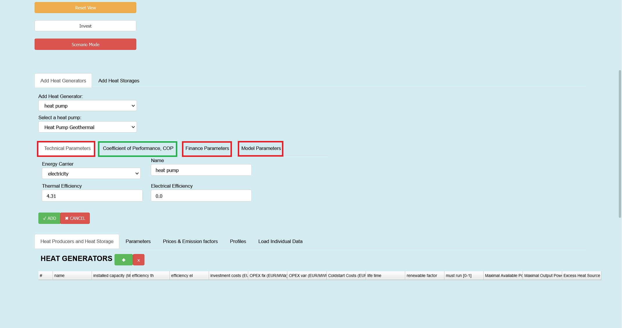
Fig. 2.31 Section for heat generator adding

By pressing the + button in the Heat Generators Table the section in Fig. 2.31 pops up (please be patient this will take some time). All heat generators have the three red marked tabs in common, only for heat pumps an extra tab is shown (Coefficient of Performance, COP; marked in a green box).

Fig. 2.32 shows you all predefined heat generator types, that means by selection one of these, predefined values are loaded. You can see and edit the values in the Technical Parameters tab and in the Finance Parameters tab, but you can also change them later in the Heat Generator table, after pressing ✓ ADD. Fig. 2.32 until Fig. 2.43 shows all possible selections and predefinitions you can make.

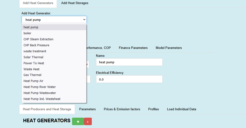
Fig. 2.32 Available heat generators to choose

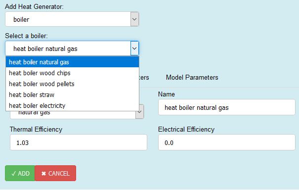
Fig. 2.33 Available types of boilers to choose

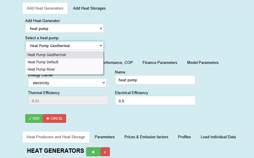
Fig. 2.34 Available types of heat pumps to choose

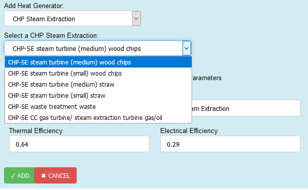
Fig. 2.35 Available types of CHP-Steam Extraction types to choose

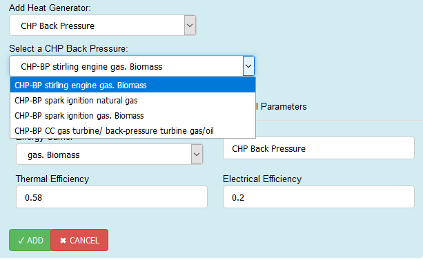
Fig. 2.36 Available types of CHP-Back Pressure types to choose

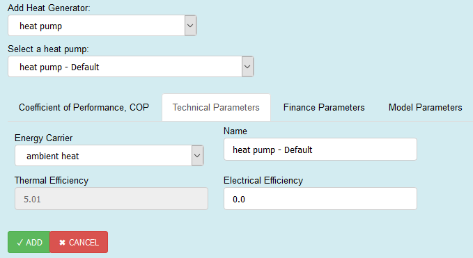
Fig. 2.37 Available types of technical parameters for heat generators to choose

In Fig. 2.37 you can select the energy carrier with which the heat generator is fired. You can define a name and set the thermal and electrical efficiency. For heat pumps the input for Thermal Efficiency is disabled, because it is defined via the Coefficient of Performance, COP tab. Each heat generator has predefined values that are shown here. You can and should change them.

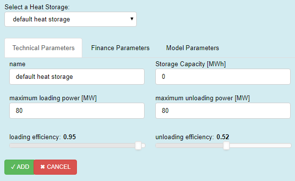
Fig. 2.38 Available types of technical parameters for heat storages to choose

In Fig. 2.38 you can define the technical parameters for your heat storage

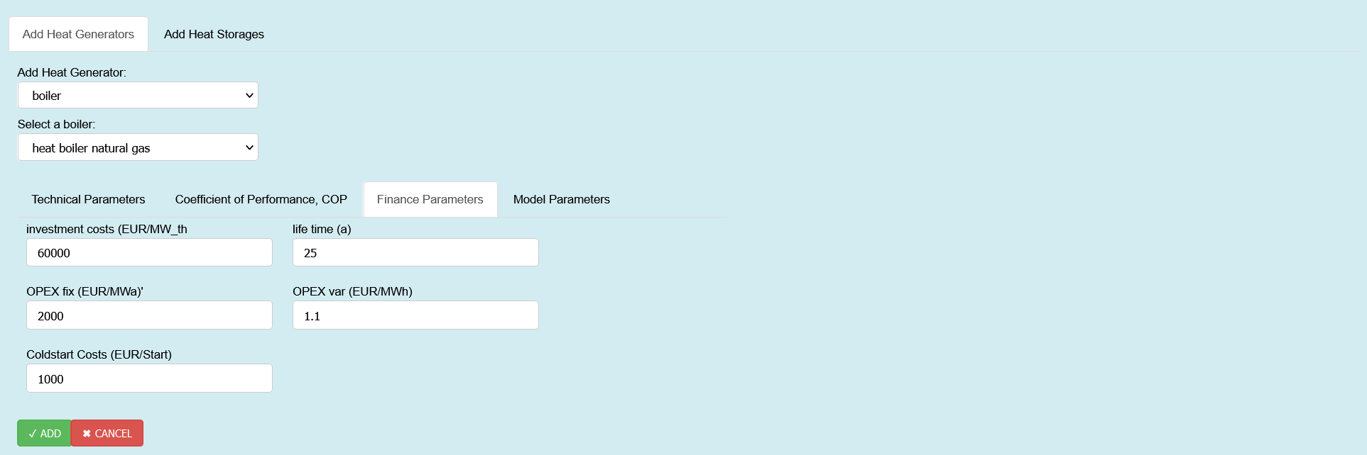
Fig. 2.39 Available types of Finance Parameters for heat generators to choose

Fig. 2.39shows you which predefined values of financial parameters for selected heat generator you can modify or in general see.

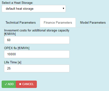
Fig. 2.40 Available types of Finance Parameters for heat storages to choose

In Fig. 2.40 you can set the financel paramters for your heat storage.

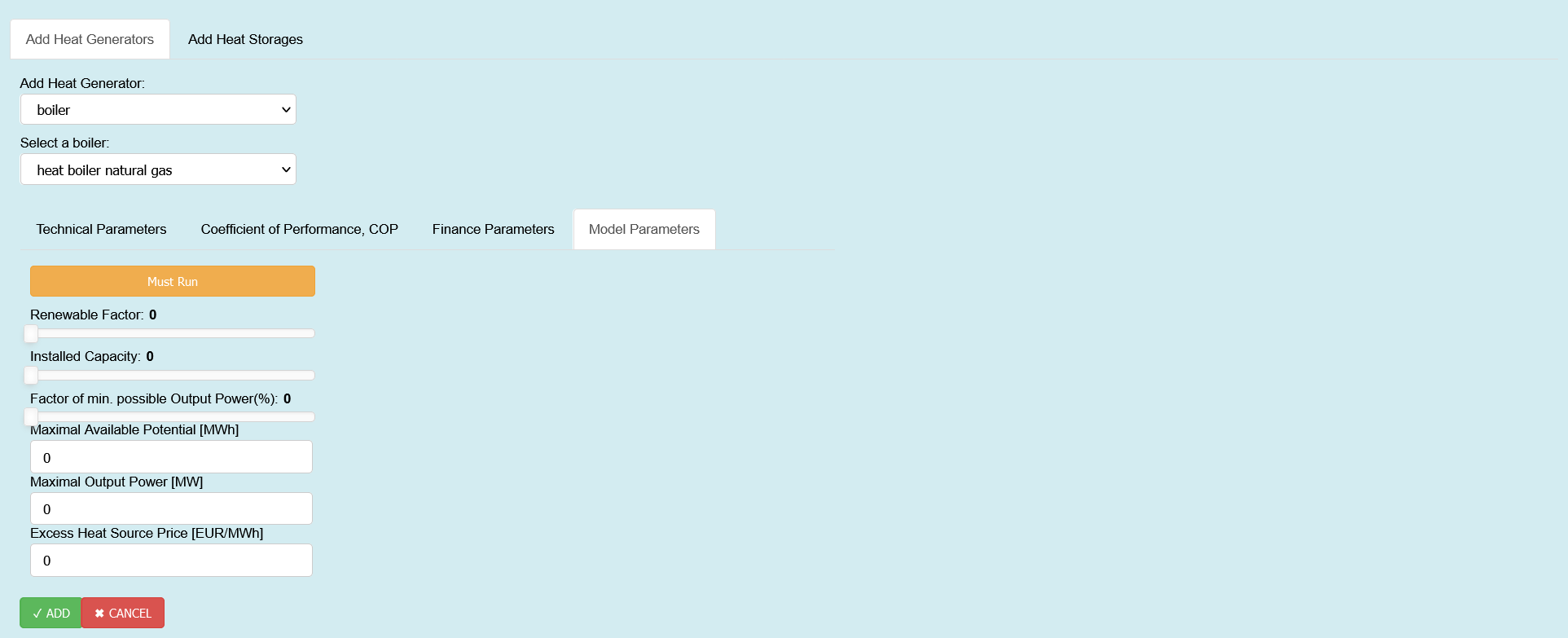
Fig. 2.41 Defining model parameters for heat generators

In this tab, shown in Fig. 2.41, you can set the orange toggle button Must Run. That mean that this heat generator must run all the time with 100% of its capacity. With one slider, you can set a Renewable Factor (values from 0 to 1) and with the other you can set the Installed Capacity of your heat generator (values from 0 to Pmax, the Peak Load of the selected Heat Profile). Beside that, you can define other parameters like Maximum Available Potential [MWh], Maximum Output Power [MW] or the Excess Heat Source Price [€/MWh].

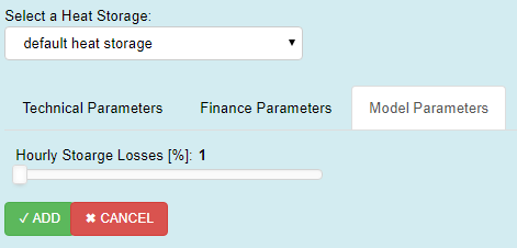
Fig. 2.42 Defining model parameters for heat stortages

In Fig. 2.42, you can set heat storage losses.

Tip

Please specify losses, because if losses are zero, it can happen that the storage is loading and unloading at the same time!

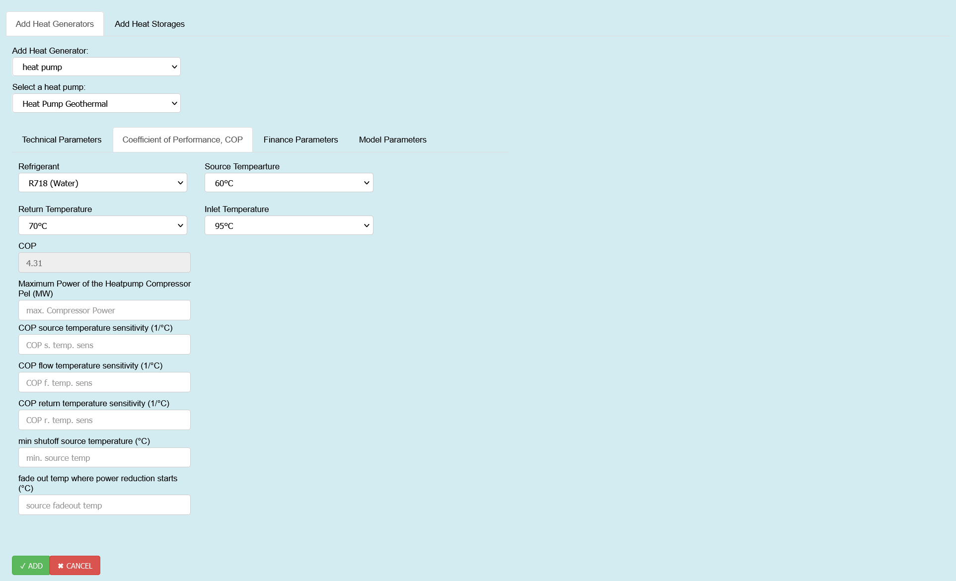
Fig. 2.43 Defining COP (only for heat pumps!)

Note

Only heat pumps have this additional tab!

Here you can select an* Inlet and Return Temperature* and, based on that selection, a COP is defined. In the Technical Parameters tab the COP value is inserted into the thermal efficiency input widget (the widget itself is disabled, meaning you cannot edit the value here, but you can change it later in the heat generators table).

2.1.2. Parameter - Tab

Fig. 2.44 Available parameter values to modify

Parameters in the table below, or also shown in Fig. 2.44, can also be changed via uploading. Therefore, you have to create an excel sheet with the structure as described in The Web User Interface (subchapter Button Section). Then the parameters must be specified in the Data worksheet.

column name	format	unit	description
CO2 Price [€/\(t_{C0_2}\)]	Number	€/\(t_{C0_2}\)	\(CO_2\) -Certificate Price (used for the short run marginal costs)
Interest Rate [0-1]	Number (real number between 0 and 1)	-	interest rate (for investment planning)
Minimum Renewable Factor [0-1]	Number (real number between 0 and 1)	-	minimum renewable share that the thermal generation should have
Total Demand[ MWh]	Number	MWh	Heat Consumption of one year; this will change the peak load (can be seen in the notification section). This cell and the Set Total Demamd (MWh) input widget in the Heat Demand Tab are coupled, this means changing one value of them changes also the other

(section: PriceAndEmissionFactors)=

2.1.3. Price & Emission factors - Tab

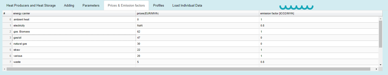
Fig. 2.45 Available prices and emission factors to modify

In general, you can set prices and emission factors for different energy carriers, like shown in Fig. 2.45. These prices are used to calculate the short run marginal costs. These parameters, as described in the table below, can also be changed via uploading. Therefor you have to create an excel sheet with the structure as described in The Web User Interface (subchapter Button Section). Then the parameters must be specified in the prices and emmision factors worksheet.

Tip

With the uploading method, you can create your own energy carriers (max. 13). If you create new ones don’t forget to specify the new names to your heat generators in the Energy Carrier worksheet.

column name	format	unit	description
energy carrier	String	-	name of the energy carrier
prices(€/MWh)	Number	€/MWh	energy carrier price
emission factor [\(t_{C0_2}\)/MWh]	Number	\(t_{C0_2}\)/MWh	\(CO_2\) -emission factor of the energy carrier

2.1.4. Radiation - Tab

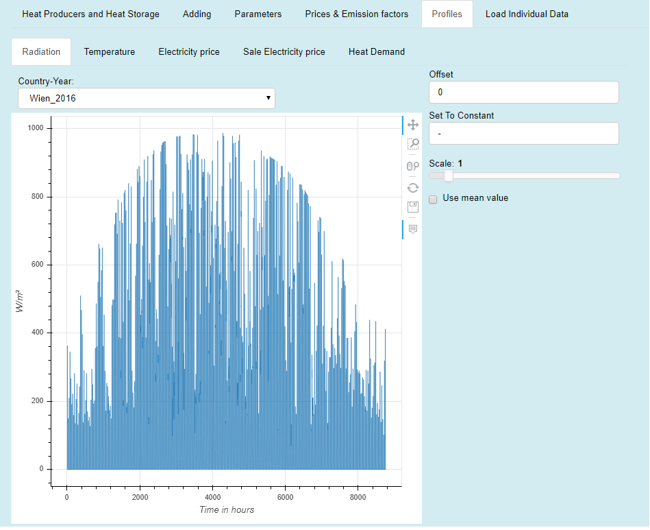
Fig. 2.46 Radiation tab

• In this tab, like shown in Fig. 2.46, you can select (Country-Year drop-down box) a predefined or a custom radiation profile with which you want to run the application.

• If you have created your own profile with the Load Individual Data tab the profile will show up in Country-Year drop-down box.

• The unit of the profile is W/m² and the model use this profile for the solar thermal power plants. If the radiation is larger than 1000 W/m² the plant works with its peak capacities installed .

You have the opportunity to make *reversible modifications on the profile:

• you can set an offset (every value of the profile will be added by the offset value)

• you can set the whole profile to a constant value

• you can scale the profile (multiplication by a factor)

• or you can use the mean value as constant profile

Note

By reversible we mean e.g. if you check the Use mean value checkbox and uncheck again you will get your profile back (see Fig. 2.47), the same occurs if you set a constant value and then delete this value you will get the profile back, see in contrast the irreversible modification tool in the Load Individual Data - Tab.

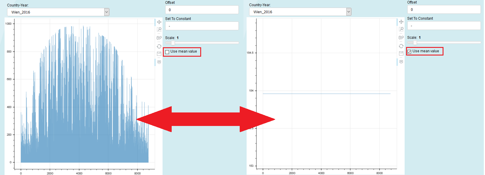
Fig. 2.47 Radiation tab and checkbox

2.1.5. Temperature - Tab

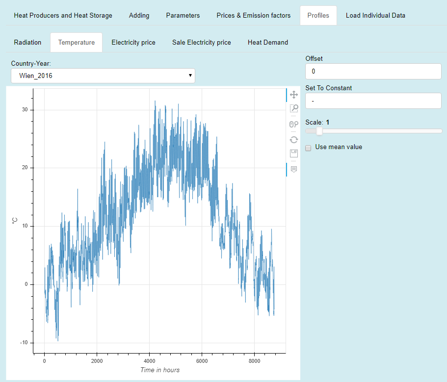
Fig. 2.48 Temperature tab

• In this tab, like shown in Fig. 2.48, you can select (Country-Year drop-down box) a predefined or a custom temperature profile with which you want to run the application.

• If you have created your own profile with the Load Individual Data tab the profile will show up in Country-Year drop-down box.

• The unit of the profile is °C and the model use this profile for the heat pumps. If the temperature is smaller than 0°C the heat pumps don’t work!

• You have the opportunity to make reversible modifications on the profile.

2.1.6. Electricity price/ Sale Electricity price - Tab

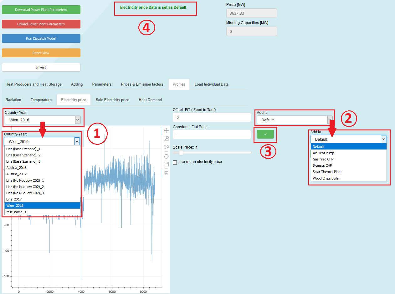
Fig. 2.49 Process to assigning a sale-/or electricity price profile

• In this tabs, e.g. the shown process in Fig. 2.49, you can select (Country-Year drop-down box) a predefined or a custom sale-/electricity price profile and then assign it to a generator (Add to drop-down box) by pressing the ** ✓** button.

• If you have created your own profile with the Load Individual Data tab, the profile will show up in Country-Year drop-down box .

• The unit of the profile is €/MWh and the model uses this for multiple purposes, e.g: if the energy carrier is electricity; this influences the short run marginal costs

• If your generator produces electricity, this affects the revenues

• Also, here you have the opportunity to make reversible modifications on the profile.

Warning

It is important to press the ✓ button, because only so changes take effect!

E.g. let’s say we want to change the default electricity price (see ):

1. Select a new profile with the Country-Year drop-down box

2. Select Default in the Add to drop-down box

3. Press the ✓ button

4. Information in the notification section will appear

Warning

This is the only way to assign a price profile, otherwise the initial profile or the last set profile is used!

2.1.7. Heat Demand - Tab

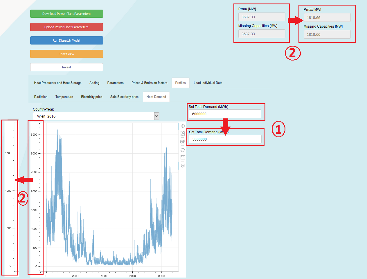
Fig. 2.50 Process to assigning a heat demand profile

• In this tab, shown in Fig. 2.50, you can select (Country-Year drop-down box) a predefined or a custom load profile with which you want to run the application.

• If you have created your own profile with the Load Individual Data tab, the profile will show up in Country-Year drop-down box .

• The unit of the profile is MW and the model use this profile as the hourly heat demand curve.

You have the opportunity to set the total heat consumption of one year. By this you set technically the sum of all values of the profile selected.

This means, if the Set Total Demand (MWh) value changes, the plot will adapt so that the sum you specified is met, also the Total Demand [MWh] value in the Parameters Tab will change to the value specified (and vice versa). Additionally, in the notification section you can see how the peak load changes when you change the total heat consumption (see Fig. 2.50).

2.1.8. Load Individual Data - Tab

Upload External Data – Button

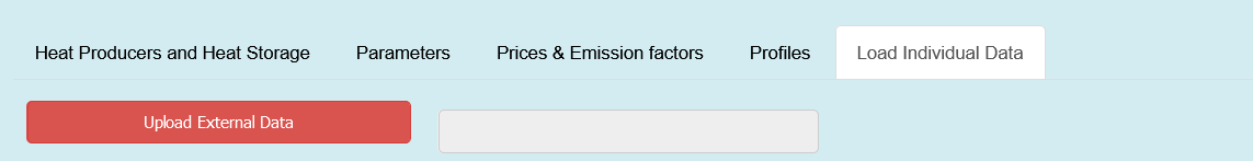
Pressing this button, shown in UploadExtData-fig, will enable you to upload your own data. A pop up window will then open, where you can select your file with the desired values. Information regarding the progress are shown in the notification section.

The file you upload must have following structure, for details see The add_profile function:

1. It has to be either a .xlsx or a .csv data

2. the files must have the structure : left: .xlsx, right: .csv)

3. you have to specify 8760 values and a header name

4. for .xlsx only the values of the first worksheet will be uploaded

An example of a successful upload can be seen in Fig. 2.51.

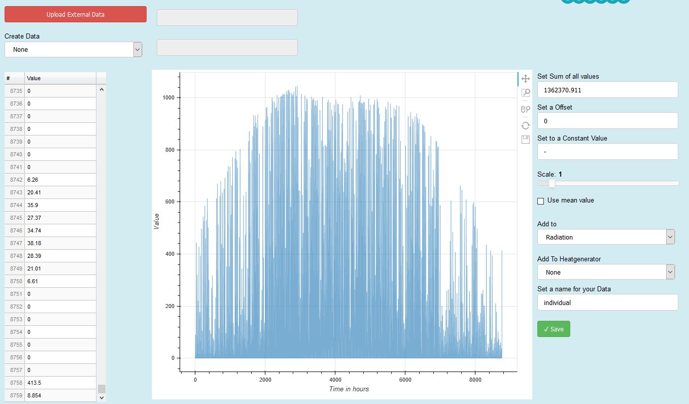
Fig. 2.51 Example of loading profile

Create Data – Tools

Here you can create random data. You can choose between three distributions (as displayed in Fig. 2.52):

1. Dirichlet Distribution

2. Normal Distribution

3. Linear Distribution

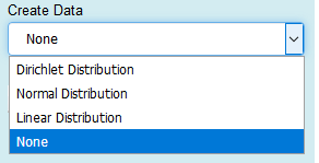
Fig. 2.52 Possible distributions

• Dirichlet Distribution:

To use this distribution, you have to specify the sum- input widget. It gives you random numbers, so the sum you specify is met. An example with the sum of 10 is shown in Fig. 2.53.

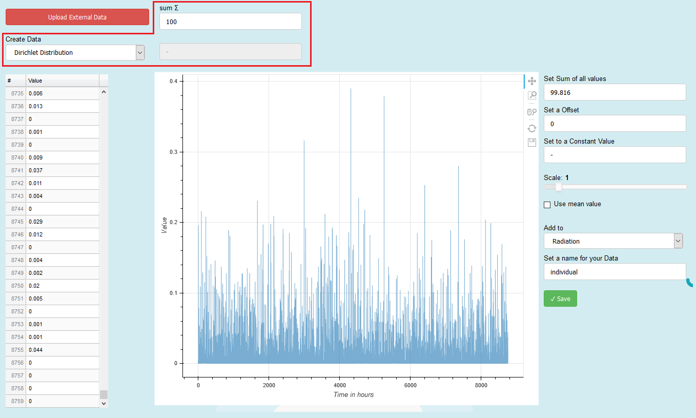
Fig. 2.53 Example of Dirichlet distribution

• Normal Distribution:

Another option to create random number is the Gaussian-Normal-Distribution. To use this, you have to specify a mean value \(\sigma\) and standard deviation from that value my \(\mu\). In Fig. 2.54, a normal distribution with \(\sigma = 100\) and \(\mu = 100\) was used.

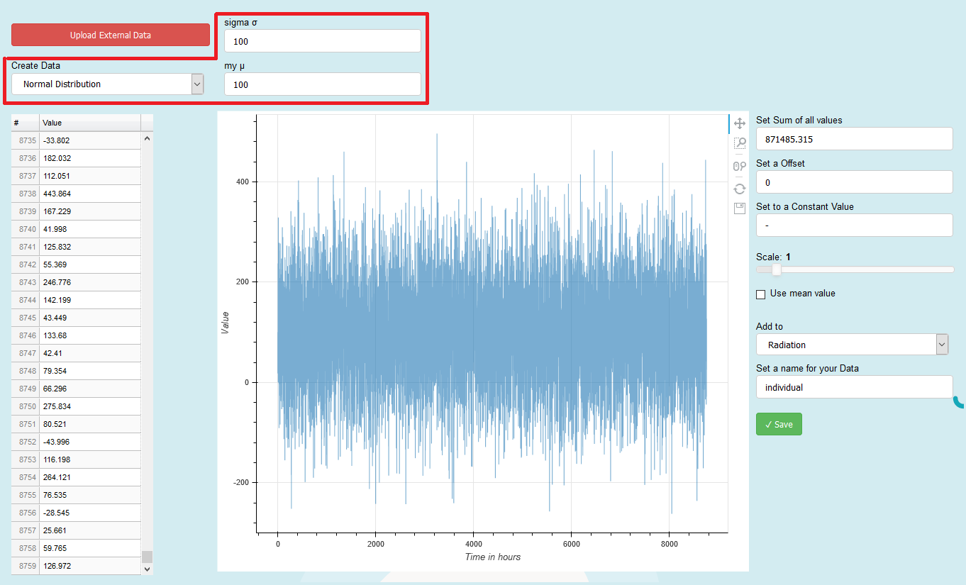
Fig. 2.54 Example of Normal distribution

• Linear Distribution:

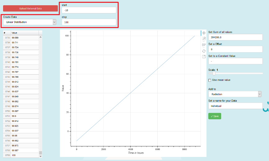
Fig. 2.55 Example of Linear distribution

With this option you can create 8760 numbers that are linear distributed beginning from start and ending with stop. An example with \(start = -10\) and \(stop = 100\) is shown in Fig. 2.55 .

Table

The values of the uploaded data or the created distribution are shown here in tabular and graphical form. You can also change specific values inside the table, in that case the cell you are editing becomes yellow and the graph is blurred. After editing, press the reset button on the toolbar to remove the blur, see Fig. 2.56.

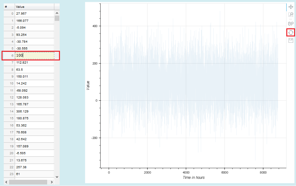
Fig. 2.56 Example of Linear distribution

Plot Area

Here a line plot of the values from the table is shown. With the toolbar at the right sight of the plot area you can inspect the data in more detail, see also Fig. 2.56.

Modification Tools

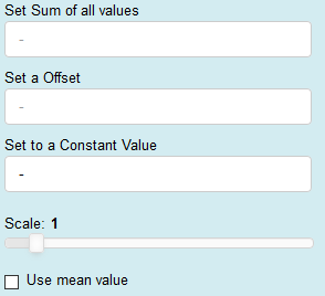
Fig. 2.57 Different modification tools

You have the opportunity to modify the data with these tools, e.g. set the sum of all values, set an offset, scale, etc (see Fig. 2.57).

Warning

This permanently change the values in the table! It works with the direct values and therefore it is an irreversible process, e.g. if you check the use the mean value checkbox and then uncheck again, you will not get your profile back, see Fig. 2.58. You have to upload or create your data again!

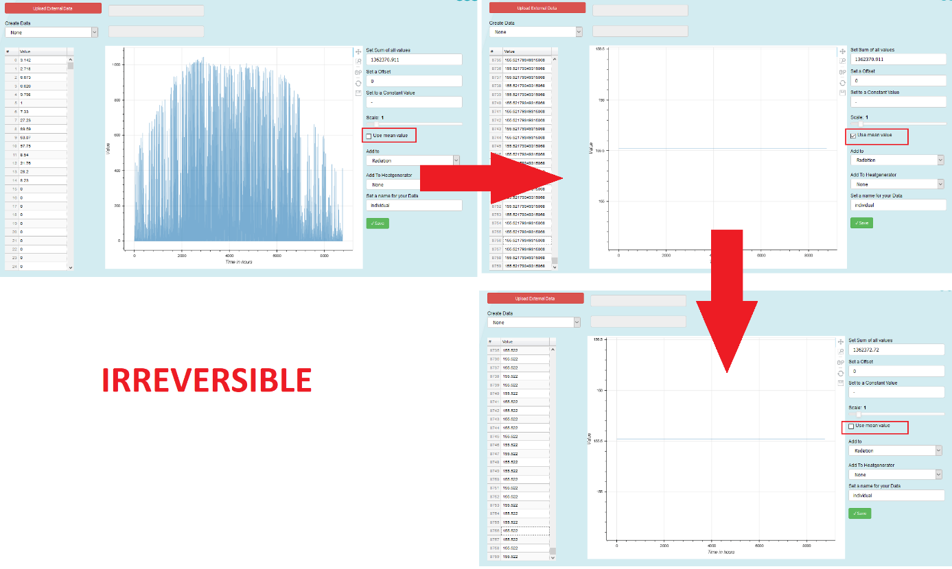
Fig. 2.58 Irreversible process of the modification tool

Saving Tools

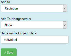
Fig. 2.59 Saving tools in general

After loading your custom data, or creating a distribution you can choose for which profile you want this dataset to be added. By pressing the Save button your data can be found at the selected profiles and can be used by selecting it with the name you specified, see Fig. 2.60.

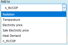
Fig. 2.60 Adding to an existing profile

Warning

The name of the data will always be terminated by the string _1 after saving (e.g. if you specify individual as your name and saved it to Radiation, you will find your profile in the Radiation Tab by the name individual_1.

It is also possible to specify a time specific thermal efficiency for a heat generator (or COP for heat pumps).

To use this feature, you have to select in the Add To drop-down button n_th/COP and then select the heat generator, Add To Heatgenerator, which you like to add your custom thermal efficiency. Then you press Save and you get an information in the notification section. Fig. 2.61 shows an example.

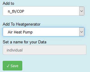
Fig. 2.61 Example of saving

2.2. How to add inputs

To be able to add new profiles, there are different script files where you can fill up the profiles.

2.2.1. Predefined script files

There are several predefined script files which can be used to pick the wanted data out of any other sources and then automatically a corresponding dat_file will be created:

• electricity_price.py: is used to generate prices by a fixed routine

• hotmapsloadprofiles.py: all parameters can be chosen individually, only the parameter nuts_code is defined by the specified load profile, depending on the NUTS2 region. Hotmaps profiles are generic profiles, hence you can define the ratio of room temeprature and hot water and the profile will be scaled individually, depending on the ratio. Additionally, with the parameter savings, you can adapt savings through room temeprature

• load_profiles.py:

• river_water_temperature.py:

• system_temperatures.py:

• pvgis_rad_temp2dat.py: pvgis data can be picked only by adding the geographical position and a name has to be chosen

• monthly_data.py: to convert automatically daily values into hourly values

The main script file which can be used to add profiles in general is readWriteDatFiles.py. Compared to other scripts, here you have to create a routine which gives you a fitting vector for adding profiles. The function which is used there is described in detail in The add_profile function.

2.2.2. Steps before add_profile function

It is important, when using the readWriteDatFiles.py, to create a routine which converts the data to an array with hourly values, therefore an array with the length of 8760, as the data itself can be only daily or other non fitting units. This numpy array will be the input of the parameter profile (see The add_profile function for detailed description of the parameters).

First, you have to get the path from the source of your data (e.g.: path of excel file, pdf document or other). Together with this path, you can use the function load_profile, where you can get the data, but first with the type pandas.series. This type of array has to be converted be able to use the data. By adding .values, the array gets the necessary data type (numpy.ndarray).

2.2.3. The add_profile function

To add a profile through the function add_profile, go to readWriteDatFiles.py , like shown in Fig. 2.62.

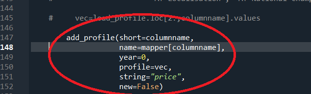
Fig. 2.62 The add_profile function

Parameters in add_profile, which have to be filled correctly:

• short: Here should be the name of your profile, but only as a short version. This name then will represent your profile when you want to choose one for calculating.

• name: This is the ful name of your profile.

• year: Choose the year where the profile is referred to.

• profile: the correct array has to be here, which will be defined before the function (see Steps before add_profile function)

• string: There you can only choose between the existing dat file types where you want to add your profile, like described in the readWriteDatFiles.py or in Fig. 2.63

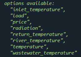
Fig. 2.63 Options for current dat files

Tip

If you don’t choose a right category, then an error will occur that you only can choose between existing dat file types.

• new: Here you can choose between boolean parameters like TRUE or FALSE. Choose FALSE, if you have many dat-files, so that the function will not overwrite the dat-files before, otherwise, if you only want to create one dat-file, then choose TRUE. .

Note

The parameters string and year are used to name the profile type with a short name like string#year. This will be important when using scenario generation and naming in excel files as it gets a better overview, see Scenario Generation.

Then run the code, if all parameters are set correctly, and by restarting the program the profile will be added in the chosen dat-file category, made by the parameter string.

1. Get started 3. Outputs